Engineering Page
Engineering
Page
On This Page
Finite Element Analysis of Structures
The Engineer's Golden
Rule:
Never use a
1/4 inch bolt where a 1/2 inch bolt will do!
Before retiring in 1990, I worked at the Lawrence Livermore National Lab for 30 years. The last few years I was the Advanced Engineering Analysis Group Leader in Weapons Engineering Division. We analyzed very complex structures. Physics developed the concepts and engineering made them deliverable. It was a great job and it was rewarding to help win the Cold War. Before becoming group leader, the last weapon system I worked on was the B-83. See a web page on the B-83 and here This is a page on Deployment.
![]()


BULLET IMPACT.... Here is a 38 special lead bullet traveling at 1000 fps impacting a 1/2" aluminum 1100-O plate. The aluminum plate is 5" in diameter and is free to translate, simulating its being supported by a string. The first view is at the time of contact. The second view is after about half of the bullet's energy has been dissipated. The third view is when about 90% of the energy has been delivered to the plate. The 4th view is a close up showing the bullet's mesh detail and the fringes of stress. The calculation halts at this point because the mesh has distorted too much to continue without rezoning. This calculation using John Hallquist's DYNA2D code took about 5 minutes on my Pentium 200 MMX computer.
CONSULTING.... I have my Pentium 200 MMX computer setup for Finite Element calculations. It boots up in DOS ready to make 2-D and 3-D meshes and run the NIKE and/or DYNA calculations. If you have a difficult structural problem that needs to be analyzed and/or redesigned, I can give you a preview of what can be done and an estimate of the cost. I can be contacted via Email.
![]()
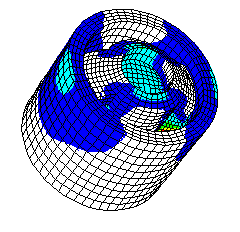
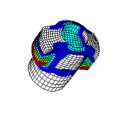
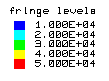
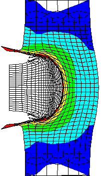
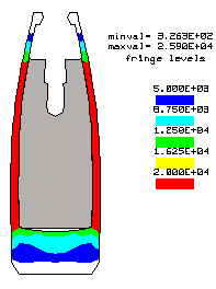
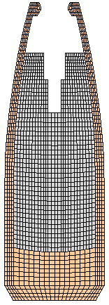
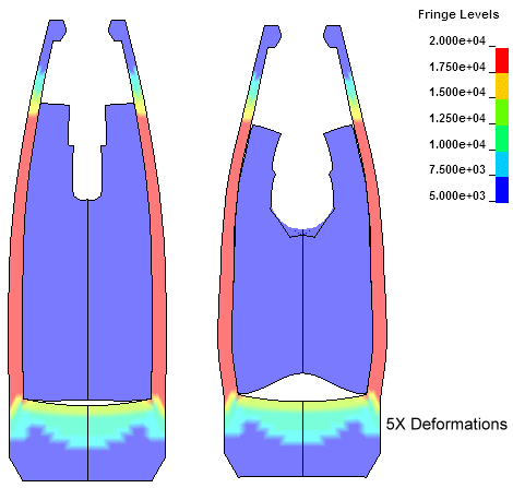
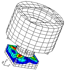
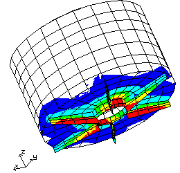
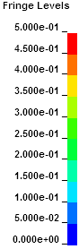
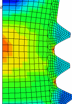
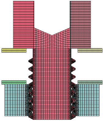
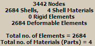
STOLLE PANDA ACTION.... Here is an example 3D Finite Element Analysis using John Hallquist's NIKE3D Finite Element Code. The stress levels in a 6-PPC caliber Stolle Panda benchrest rifle action are shown at a peak internal chamber pressure of 50,000 psi. This pressure occurs during firing when the bullet has only traveled a short distance down the barrel. I have updated the calculation with the latest LS-DYNA Finite Element Code. Click Here to view the updated results. The first Figure shows the action with the bolt in the locked position. The second Figure shows only the bolt where the maximum stress level, in the lugs, is 87,700 psi. The third Figure is the action with a maximum stress level of only 41,300 psi. Note that the high stressed region of the bolt is in compression and occurs at the area of contact with the action. The stress levels are in psi, see the legend. To run this calculation out to seven time steps, took about 2 hours of number crunching. FEA Publications published my analysis in the .pdf format. Click here to view the publication.
A more detailed analysis of the Stolle Panda action stresses and
deflections here.
This is a animated deformation view as the pressure increases from
0 to 50,000 psi in 5,000 psi steps. The 243 Win brass has a
friction coefficient of 0.41 between the brass and the 416
stainless steel chamber. The fringes are of effective plastic
strain. Note that the primer backs out at first and then is
reseated. The detailed calculation is here.
![]()
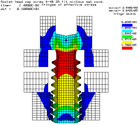
BOLT ANALYSIS.... I worked for many years at the Lawrence Livermore National Laboratory performing engineering structural analysis on complex systems. The example calculation above is a 2D Finite Element Analysis of a 4-40 socket head cap screw being loaded to its breaking point and the resulting stress levels. The FEA software used was John Hallquist's NIKE2D Finite Element Code. The number crunching took about 10 minutes of CPU time on my P5-200 MMX computer. See the new bolt load analysis with LS-DYNA here.
![]()

![]()
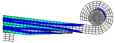
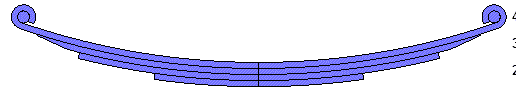
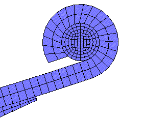
TRUCK LEAF SPRING.... Above is an example of a truck leaf spring analysis using John Hallquist's NIKE2D with the plane strain option. The first view is the spring mesh outline in the unloaded condition. There are slide surfaces between the leaves and between the end coils and the shafts. The slide surfaces transmit compressive loads, and allow sliding with friction. The second figure shows the stress levels with the spring deflected 5 inches. The third Figure is a close up view of one end, showing the mesh detail. The shaft is not allowed to rotate, and the spring coil rotates around the shaft with a 0.1 coefficient of friction.
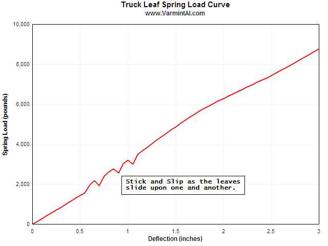
LOAD DEFLECTION CURVE.... I modeled the Truck Leaf Spring in
3D and ran an implicit quasi-static calculation with LS-DYNA to calculate the
load deflection characteristics of the spring. Notice that during
the early deflections there is some stick and slip as the leaves
contact each other.
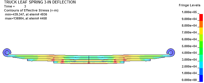
FULLY LOADED.... Here the spring is deflected 3" at the
center and the load is 8600 pounds. The stress is high and it would
be lower if the short leaves had tapered ends. The end pins are
allowed to move horizontally since the spring increases its length
when loaded. Very high stresses would occur if the ends were
prevented from moving to allow for the increased spring length.
MOVIE.... Here is an animation of the deflection and stress
levels as the spring is loaded.
CONTACT SURFACE.... This clip shows the motion as the spring
increases its length and rotates around the end pin. The end pin is
allowed to move to the right, but restrained both from rotation and
moving vertically. If the link system in mounting the spring
did not allow the increase in length the stresses in the main leaf
would be very high.
![]()


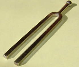 TUNING FORK.... I measured a steel 440 Hz
tuning fork (note "A" on the music scale) with a dial caliper to
determine the dimensions for a 2D finite element plane stress model
with a 0.155 inch thickness. A plane strain model (infinitely long
normal to the above views) was less accurate in predicting the
correct mode frequency. I used the NIKE2D Finite Element
code for the modal analysis. The blue tuning fork in its rest state
and red views show the first 5 natural frequency mode shapes. The
handle of the tuning fork was not modeled since is is merely a way
to hold the tuning fork without dampening out the vibrations. Using
the average measurements of the geometry and properties of 4140
steel, the mode 1 accuracy is within 3.2%. The frequencies are:
TUNING FORK.... I measured a steel 440 Hz
tuning fork (note "A" on the music scale) with a dial caliper to
determine the dimensions for a 2D finite element plane stress model
with a 0.155 inch thickness. A plane strain model (infinitely long
normal to the above views) was less accurate in predicting the
correct mode frequency. I used the NIKE2D Finite Element
code for the modal analysis. The blue tuning fork in its rest state
and red views show the first 5 natural frequency mode shapes. The
handle of the tuning fork was not modeled since is is merely a way
to hold the tuning fork without dampening out the vibrations. Using
the average measurements of the geometry and properties of 4140
steel, the mode 1 accuracy is within 3.2%. The frequencies are:
Mode 1    454 Hz
Mode 2  2,850 Hz
Mode 3  7,513 Hz
Mode 4 10,947 Hz
Mode 5 16,657 Hz
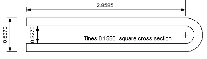
The tuning fork is made of steel with a modulus, E = 29 msi,
Poisson ratio = .29 rho = .283 lb/in^3
These are the dimensions measured from the tuning fork. See how
accurately your software calculates Mode 1.
THREE DIMENSIONAL MODEL.... The Tuning Fork modal analysis was repeated using LS-DYNA with a 3-D mesh. Here are the first 4 modes shown in animated gif files.
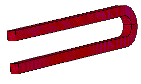 Mode 1 at 450.44 Hz (2.3% Error) |
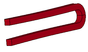 Mode 2 at 2823 Hz |
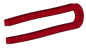 Mode 3A at 7460 Hz |
 Mode 4 at 8438 Hz (torsion) |
Notice that it was not possible to identify Mode 4 (a rotational twisting of the tuning fork tines) with the 2-D model.
HOW ACCURATE?.... How accurately do the FEA codes calculate the mode vibration frequencies? Below is a table comparing the modal frequency calculations for the first 5 mode shapes of a steel cantilever beam with a 0.5" square cross section and a length of 20". The equation in Chapter One, from the Shock and Vibration Handbook (Third Edition) should be quite accurate since it uses a "fudge factor" for each mode to normalize the results to test data.
This view of the 0.5" square beam is Mode #3 at 700 Hz. The left end condition is fixed to a rigid wall. For the LD-DYNA 3-D calculation, the 5000 elements were 0.1" cubes and in *SECTION_SOLID the ELFORM was set at 18 (8 point enhanced strain solid element for linear statics only).

 Mode 1 40.19 Hz |
 Mode 2 251.2 Hz |
 Mode 3 700.1 Hz |
 Mode 4 1363. Hz |
 Mode 5 2334. Hz |
 Torsional Mode 1391. Hz |
Modal Analysis Accuracy Comparison
Mode Frequencies in Hz
Steel Cantilever Beam 0.5" x 0.5" x 20" long
| Mode Number |
Shock Handbook Equation | NIKE2D Plane Stress 1280 Elements |
LS-DYNA 3-D 5000 Elements |
| 1 | 40.2 | 40.67 | 40.19 |
| 2 | 251 | 254.1 | 251.2 |
| 3 | 705 | 708.3 | 700.1 |
| 4 | 1380 | 1379 | 1363 |
| 5 | 2280 | 2260 | 2334 |
.
|
Horizontal End Deflection |
| D=W*L^4/(8*E*I)
Classical beam equation for the end
deflection of a horizontal cantilever beam from it own weigh. Deflection calculated with LS-DYNA D = 0.00948614 (in) Error = 1.25% |
![]()
MAXIMUM SPIN VELOCITY.... This is in response to some of the BBS posts about "How Fast?" can one shoot a bullet before it will explode in midair. It turns out that it is not how much velocity, but rather, how fast is it spinning that counts. A bullet with a thicker jacket will withstand higher spin velocities than the bullet I selected to model, but here are the results of the analysis.
I have done a 2D Finite Element calculation of the spin velocity necessary to fail a .224" 40 gr. bullet with a 0.012" gilding metal jacket wall and a pure lead core. The yield stress used for the gilding metal (G21000 95Cu/5Zn) was 15 KSI. At a spin velocity of 307,500 rpm a condition of plastic instability occurs. The bullet's jacket begins to yield and the radius increases. This increase of radius puts an even higher stress on the jacket, but the jacket metal is strain hardening. Instability occurs when the radius increases at a greater rate than the jacket is strengthened due to strain hardening. The Finite Element Code could not find an equilibrium position for the next increment of spin velocity and terminated. Therefore, from the calculation, this bullet would fly apart at or near 307,500 rpm. Using this as the maximum spin velocity capability, the following are the twist rates (inches for one turn) and the associated muzzle velocity to fail this bullet:
Twist = 7 Max Vel = 2989
fps
Twist = 8 Max Vel = 3416 fps
Twist = 9 Max Vel = 3843 fps
Twist = 10 Max Vel = 4270 fps
Twist = 11 Max Vel = 4697 fps
Twist = 12 Max Vel = 5124 fps
Twist = 13 Max Vel = 5551 fps
Twist = 14 Max Vel = 5978 fps
Twist = 15 Max Vel = 6405 fps
Twist = 16 Max Vel = 6832 fps
 Mesh outline. |
 Deformations amplified 20X. |
 Effective stress. |
The first Figure is the outline and detail of the Finite Element mesh. The second Figure is of the deformations, amplified by 20X, at 307,500 rpm. The third Figure is the effective stress levels in the jacket gilding metal at 307,500 rpm and it shows that most of the cylindrical section of the bullet is stressed above the 15 KSI yield stress. The maximum stress is 16.46 KSI. Any damage done to the bullet during firing, such as engraving of the jacket and deformations due to torsional impulse will only reduce the bullet's spin velocity capability.
Here is the same calculation as above performed in 2D with LS-DYNA.
The deformations are amplified by 20X for the effective stress
view. A much finer mesh was used and the calculation took about 1
minute to complete. With the old NIKE2D code running on a 486
computer the calculation took about 30 minutes.
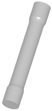
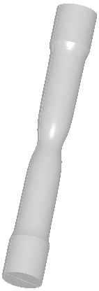
NOSLER BULLET.... This is a 2D Finite Element analysis, using the NIKE2D code, of a spinning .243" 55 gr. Nosler Ballistic Tip bullet. One would think that a bullet with a larger diameter would have less spin velocity capability than a smaller bullet. But this bullet design with the same material properties as the .224 bullet above, fails at 420,000 rpm. The good people at Nosler have cleverly strengthened the bullet to withstand high spin velocities. The first improvement is that the solid base has enough thickness so it does not dish in from the high powder pressures or after exit when the jacket wants to expand radially. Note that the base of the .224 bullet is concave. The solid base also minimizes the radial expansion of the jacket near the base. The second feature is the thick boss at the jacket mouth which provides hoop strength to reduce radial expansion. I did not include the plastic nose tip in the calculation. It is such a light material and the diameter is so small that it would put only a very small radial loading on the jacket nose. But plastic nose tip's presence during flight prevents the in flight stagnation gas pressure from radially forcing open the nose of the jacket. All of these features combined make a very stable bullet for surviving high spin velocities. Using 420,000 rpm as the maximum spin velocity capability, the following are the twist rates (inches for one turn) and the associated muzzle velocity to fail this bullet:
Twist = 7 Max Vel = 4083
fps
Twist = 8 Max Vel = 4667 fps
Twist = 9 Max Vel = 5250 fps
Twist = 10 Max Vel = 5833 fps
Twist = 11 Max Vel = 6417 fps
Twist = 12 Max Vel = 7000 fps
Twist = 13 Max Vel = 7583 fps
Twist = 14 Max Vel = 8167 fps
Twist = 15 Max Vel = 8750 fps
Twist = 16 Max Vel = 9333 fps
 Mesh Unloaded |
 Deformed times 5X |
 Stress levels at 420,000 rpm |
The first Figure is the FEA mesh detail in the unloaded condition. The second Figure is the deformations that occur at 420,000 rpm just before failure with the deformations amplified by 5X. Note that the solid base does not undergo the concave deformations of the thin based bullet above and remains flat. The soft lead core is radially forced outward against the jacket and the nose opening diameter of the jacket remains almost unchanged. The third Figure shows the stress levels in the jacket and a stress of 25.9 KSI is reached before the bullet fails. This, in my opinion, is a very well thought out bullet design.

Here is the same calculation as above performed in 2D with LS-DYNA.
The deformations are amplified by 5X for the effective stress view.
A much finer mesh was used and the calculation took about 1 minute
to complete. With the old NIKE2D code running on a 486 computer the
calculation took about 30 minutes. Note that with the finer mesh
the distortions at the center of the cavity in the lead core the
outline overlaps the mesh. This does not occur but is due to the 5X
amplifications of the displacements.
![]()
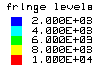
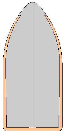
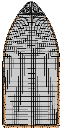
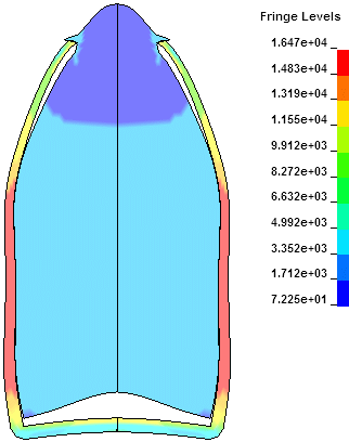
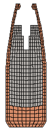
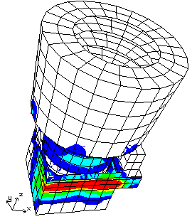
STAR TRACKER CAMERA.... Here is an example Finite Element Analysis using John Hallquist's NIKE3D. The Star Tracker Camera body and baffle are exposed to 100 G's of X Acceleration and the resulting stress levels are shown. In the second view, the baffle is removed from the camera
body and rotated 180� for better viewing. The stress levels were also calculated for Y, and Z acceleration. The Z axis is parallel to the axis of the baffle. Using, the same model, composed of mostly shell elements, a modal analysis was done to calculate the natural frequency of the first 8 modes of vibration.![]()

UV/VISIBLE CAMERA.... Here is another example of Finite Element Analysis using NIKE3D. The UV/Visible Camera body and baffle are exposed to 100 G's of Y Acceleration and the resulting stress levels are shown. In the second view, the baffle is removed from the camera body and rotated 180� for better viewing.
![]()
FREE SOFTWARE.... If you have made it this far, there is a reward! Here are two FREE engineering tools that I have used over the years. The first one, BOLTS.ZIP (34K) is a bolt calculator program that calculates how many bolts are required to withstand a given axial load with a specified yield safety factor. The code includes most bolt material properties and bolt data for sizes from 0-80 up to 1-1/2"-6 and for both NC and NF threads. If a bolt circle diameter is specified, it will display a CGA scale drawing of the bolt pattern. Want to forget about DOS? See the new Bolt Calculator below.
![]() NEW BOLT CALCULATOR.... Paul Bussieres has ported the old
DOS Bolt Calculator program over to Visual Basic 6.0. He has done
an excellent job keeping it small plus all the instructions are
right on the screen. I have checked it out and it works well and is
much easier to use than the old DOS version. Click on boltsvb.zip (33K)
NEW BOLT CALCULATOR.... Paul Bussieres has ported the old
DOS Bolt Calculator program over to Visual Basic 6.0. He has done
an excellent job keeping it small plus all the instructions are
right on the screen. I have checked it out and it works well and is
much easier to use than the old DOS version. Click on boltsvb.zip (33K)![]() and download the file to a temp folder on
your compute. No installation is required. When you unzip it, it
will create a C:\BoltsVB folder and put two files in that folder,
the executable and an icon file.. Use your Find command and look
for boltsvb.exe on your C: drive. Right click on boltsvb.exe and
create a icon on your desktop or double click on boltsvb.exe and
calculate the number and size of bolts to support a given load. If
you don't like the program, merely delete the bolts folder on your
C: drive. There are no other files added to your computer.
and download the file to a temp folder on
your compute. No installation is required. When you unzip it, it
will create a C:\BoltsVB folder and put two files in that folder,
the executable and an icon file.. Use your Find command and look
for boltsvb.exe on your C: drive. Right click on boltsvb.exe and
create a icon on your desktop or double click on boltsvb.exe and
calculate the number and size of bolts to support a given load. If
you don't like the program, merely delete the bolts folder on your
C: drive. There are no other files added to your computer.
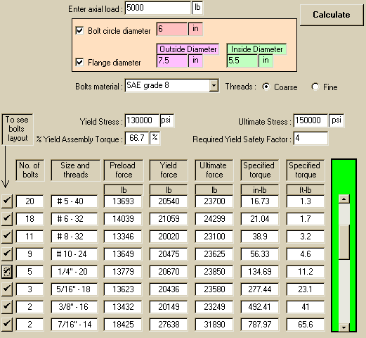
Screen view of the boltsvb.exe calculation for an axial load of
5000 lb and using bolts
made of Grade 8 steel. Once the user selects a bolt size, then he
can specify how many
bolts to use.
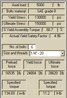
Output from boltsvb.exe after
selecting 6 bolts instead of 5.
GAS EQUATION OF STATE.... The GASB.ZIP (26K) program is the old DOS version of a gas equation of state solver. Given a temperature and any two of PRESSURE, VOLUME, or MASS, it calculates the third. The Beattie-Bridgeman Equation of State data for 10 common gases are built into the code. The solutions are reasonable for temperatures from about -60�F to 500�F. The solutions is not valid near the triple point for a given gas.
Down load the software by clicking on the name. They are zipped and must be unzipped to be used. These codes were written a long time ago and have to be run in a DOS Box. They are not pretty, but if you need to know how many bolts or the mass of the gas, they will quickly give reasonable results.
![]() NEW
GAS PROGRAM.... Paul Bussieres has done an excellent job
translating the old Gasb.exe program from BASIC to Visual Basic
6.0. Click on GasVB.zip (16K) and download
the file to a temporary folder on your compute. No installation is
required. When you unzip it, it will create a C:\GasVB folder and
puts two files in that folder, the executable and an icon file. Use
your Find command and look for GasVB.exe on your C: drive. Right
click on GasVB.exe and send a shortcut Icon on your desktop or
double click on GasVB.exe and calculate the properties of the
listed gases. If you don't like the program, merely delete the
C:\GasVB folder on your C: drive. There are no other files added to
your computer.
NEW
GAS PROGRAM.... Paul Bussieres has done an excellent job
translating the old Gasb.exe program from BASIC to Visual Basic
6.0. Click on GasVB.zip (16K) and download
the file to a temporary folder on your compute. No installation is
required. When you unzip it, it will create a C:\GasVB folder and
puts two files in that folder, the executable and an icon file. Use
your Find command and look for GasVB.exe on your C: drive. Right
click on GasVB.exe and send a shortcut Icon on your desktop or
double click on GasVB.exe and calculate the properties of the
listed gases. If you don't like the program, merely delete the
C:\GasVB folder on your C: drive. There are no other files added to
your computer.
|
Equation of State data included
for: |
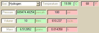
Sample screen shot for calculating Hydrogen, given there was 100
psi
in a 10 liter container. The code calculates the mass. Then see
below.
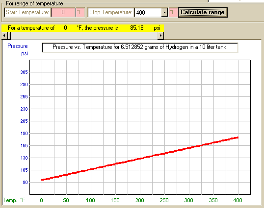
The code also calculates the pressure change for a range of
temperatures that are user selected.
![]()
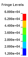
MATERIAL PROPERTIES DATABASE.... I have included a material.txt Database of over 1000 structural materials. The properties are in English Units. These are the data that I have use for years as input to the Finite Element calculations. Below is a sample of the data for the first eight entries. The system of units is:
Updated 5/22/2011 |
1 ALUMINUM PURE 99.996 ANNEALED 0.0970 10.00 0.330 1.8 7.0 50.0 --- 13.20 0.20 |
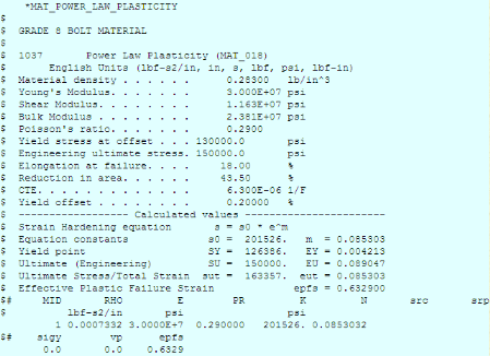
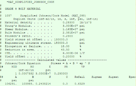
LS-DYNA USERS.... I have calculated the low strain-rate material property coefficients for all 1,044 materials in the Database so that they can be used in LS-DYNA. It started with MAT_018 (*MAT_POWER_LAW_PLASTICITY) and have expanded to include material models for MAT_024 & MAT_098. Once the files are downloaded and unzipped you can use your text editor to search for the material of interest. Comment cards are included for each material that give the mechanical properties data plus the calculated strain hardening power law parameters. Each material entry is formatted so that it can be copied from the text file and pasted directly into the LS-DYNA Keyword input file. I have made the MID (material ID number xx) and it will need to be changed to the correct value for your particular calculation.
IF A MATERIAL IS NOT IN THE DATABASE.... If a material is not listed in the large 1044 material.txt Database, mat18.exe will calculate the Power Law Plasticity (MAT_018) and/or (MAT_098) for a single material. mat18.exe is a small executable file that will run in DOSBOX on a Linux operating system. The input is entered from the keyboard and the out put file is in the correct format for insertion into an LS-DYNA Keyword input file. English units are used and it is up to the user to convert to the desired units.| $
================================================================== *MAT_POWER_LAW_PLASTICITY $ $ Alumin - 6061-T6 $ $ Power Law Plasticity (MAT__018) $ English Units (lbf-s2/in, in, s, lbf, psi, lbf-in) $ Material density . . . . . . 0.09800 lb/in^3 $ Young's Modulus. . . . . . . 1.000E+07 psi $ Shear Modulus. . . . . . . . 3.759E+06 psi $ Bulk Modulus . . . . . . . . 9.804E+06 psi $ Poisson's ratio. . . . . . . 0.3300 $ Yield stress at offset . . . 42200.0 psi $ Engineering ultimate stress. 44900.0 psi $ Elongation at failure. . . . 16.50 % $ Reduction in area. . . . . . 50.00 % $ Yield offset . . . . . . . . 0.20000 % $ ------------------ Calculated values ----------------------- $ Strain Hardening equation s = s0 * e^m $ Equation constants s0 = 54943. m = 0.050692 $ Yield point SY = 41613. EY = 0.004161 $ Ultimate (Engineering) SU = 44900. EU = 0.051999 $ Ultimate Stress/Total Strain sut = 47235. eut = 0.050692 $ Effective Plastic Failure Strain epfs = 0.000000 $# MID RHO E PR K N src srp $ lbf-s2/in psi psi xx 0.0002539 1.0000E+7 0.330000 54943. 0.0506919 $# sigy vp epfs 0.0 0.0 0.0000 $ ========Replace xx above with the local material I.D. number====== |
| $
================================================================== *MAT_SIMPLIFIED_JOHNSON_COOK $ $ Aluminum - 6061-T6 $ $ Simplified Johnson/Cook Model (MAT_098) $ English Units (lbf-s2/in, in, s, lbf, psi, lbf-in) $ Material density . . . . . . 0.09800 lb/in^3 $ Young's Modulus. . . . . . . 1.000E+07 psi $ Shear Modulus. . . . . . . . 3.759E+06 psi $ Bulk Modulus . . . . . . . . 9.804E+06 psi $ Poisson's ratio. . . . . . . 0.3300 $ Yield stress at offset . . . 42200.0 psi $ Engineering ultimate stress. 44900.0 psi $ Elongation at failure. . . . 16.50 % $ Reduction in area. . . . . . 50.00 % $ Yield offset . . . . . . . . 0.20000 % $ ------------------ Calculated values ----------------------- $ Johnson/Cook Equation Stress = A + B * ep ^ N $# MID RO E PR VP $ lbf-s2/in psi XX 0.0002539 1.0000E+7 0.330000 $# A B N C Psfail Sigmax Sigsat Epso $ psi psi 38700. 18395. 0.2583357 0.0 0.0000 $ ========Replace xx above with the local material I.D. number====== |
Downloads for material properties WITHOUT Effective
Plastic Failure Strain (epfs).
English Units (lbf-s2/in, in, s, lbf, psi, lbf-in)
SI Units (kg, m, s, N, Pa, Joule)
GM Units (kg, mm, ms, kN, GPa, kN-mm)
FC Units (tonne, mm, sec, N, MPa, N-mm)
PH Units (gram, cm, microsec, 107
N, Mbar, 107 N-cm)
![]() NOTE Fix
for MAT_024 and MAT_-90.... LS-DYNA does not read the "D"
double precision type exponte correctly.
NOTE Fix
for MAT_024 and MAT_-90.... LS-DYNA does not read the "D"
double precision type exponte correctly.
I have converted the example ( 1.2340D+03 type exponent over to the
1.2340E+03 type). The data is the same only the "D"
have been replaced with "E".
Power Law Plasticity (MAT_018)
Download:
mat18-all-no-failure.zip
(422 Kb) Includes epfs for all 1044 materials, 5 systems of
units.
Piecewise Linear Plasticity (MAT_024)
Download:
mat24-all-no-failure.zip
(6.14 Mb) Includes epfs for all 1044 materials, 5 systems of
units.![]()
1. Each MAT_024 includes a Defined Curve with a curve ID of
the materials list number plus 1000.
2. Each MAT_024 must include the full 101 points in the plastic
strain vs true stress Defined Curve.
Simplified Johnson Cook (MAT_098)
Download:
mat98-all-no-failure.zip
(249 Kb) Includes epfs for all 1044 materials, 5 systems of
units.
List of the 1044 Materials by I.D. Number
Download:
The matlist.txt file which lists all 1044
materials by the list I.D. number including yield and ultimate
stress.
Here are the 3D KEYWORD files setup for MAT_018 of Aluminum 6061-T6
both with and without failure.
The mesh is a 10 degree sector of the standard tensile test
specimen with boundary nodes constrained.
Download
the files here: pull3dspin-aluminum-6061-t6-run.zip
Aluminum 6061-T6 Tensile Test
Simulation with MAT_018
Power Law Plasticity Material Model
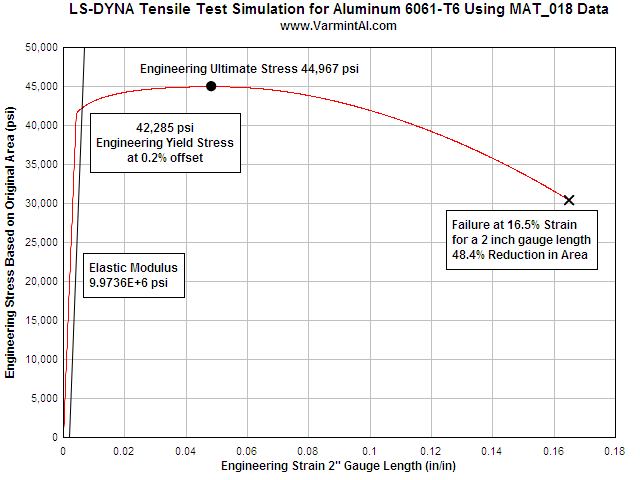
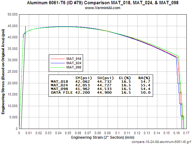
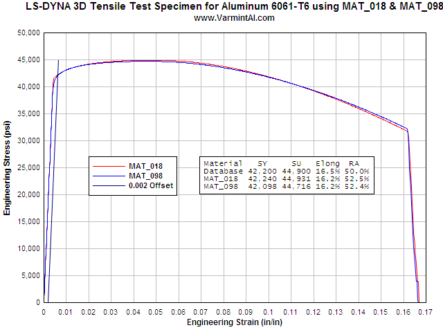
VERIFYING MAT_018.... The object of this calculation was to verify that MAT_018 would reproduce the input material data from a simulation of a Tensile Test. The FEA geometry is that of a 1/2" Standard Tensile Test that is used to measures the mechanical properties of metals. The calculation runs in the 2D implicit mode with the load applied as an extension in 0.0001 inch increments. The resulting load was then calculated with LS-PrePost using the bndout ASCII file. The mesh consists of 3,171 nodes and 2960 2D elements. The run time is about 10 minutes on my 2.6 GHz Athlon XP 64 computer. If you would like to run the calculation yourself here is the LS-DYNA Keyword input file: Download mat_018-keyword-input-files.zip (53Kb) It is setup to run with aluminum 6061-T6 but it is very easy to change the MAT_018.k file to a material of interest.
The chart shows the calculated Engineering Stress vs Strain in a two inch gauge length of the 2D LS-DYNA simulation. The Power Law Plasticity material model reproduces the input properties with good accuracy. The largest error is in the Reduction in Area. In an actual tensile test specimen measuring the diameter at the fracture location is difficult to do accurately. The tensile test simulation was also done for steel 4140. The agreement here is well within the range that is normally expected between samples of the same material.
Table 1: Comparison of the Aluminum 6061-T6 Results to the Input Material Properties
| Material Property | Input From the MAT_018 Database | LS-DYNA Calculated Property from the FEA Simulated Tensile Test | Error |
| Modulus of Elasticity | 10,000,000 psi | 9,973,600 psi | 0.26% |
| Engineering Yield Stress | 42,200 psi | 42,285 psi | 0.20% |
| Engineering Ultimate Stress | 44,900 psi | 44,967 psi | 0.15% |
| Elongation at Failure | 16.5% | 16.2% | 1.82% |
| Reduction in Area | 50% | 52.4% | 4.80% |
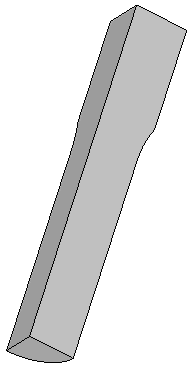
FEA Mesh and Animation of the Tensile Test for Aluminum 6060-T6
 Standard 1/2 diameter Tensile Test Specimen |
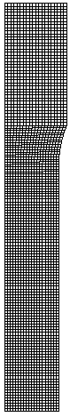 Mesh Density used in the Calculation |
 |
 Effective Stress |
Table 2: Material Property input in the Tensile Test Simulation
*MAT_POWER_LAW_PLASTICITY |
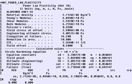
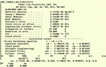
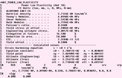
EXAMPLE.... Aluminum 6061-T6 shown in the other unit
systems.
![]()
Steel 4140 Tensile Test Simulation
with MAT_018
Power Law Plasticity Material Model
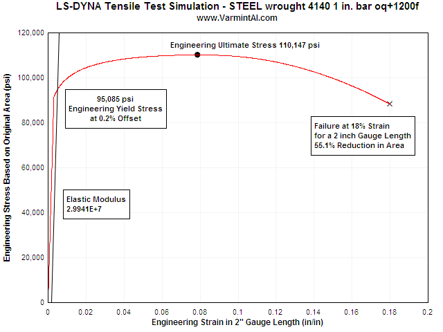
Table 3: Comparison of the Steel 4140 Results to the Input Material Properties
| Material Property | Input From the MAT_018 Database | LS-DYNA Calculated Property from the FEA Simulated Tensile Test | Error |
| Modulus of Elasticity | 30,000,000 psi | 29,941,040 psi | 0.20% |
| Engineering Yield Stress | 95,000 psi | 95,085 psi | 0.09% |
| Engineering Ultimate Stress | 110,000 psi | 110,147 psi | 0.13% |
| Elongation at Failure | 18.0% | 18.0% | - |
| Reduction in Area | 53% | 55.1% | 3.96% |
Table 4: Steel 4140 Material Property input in the Tensile Test Simulation
*MAT_POWER_LAW_PLASTICITY |
CALCULATED VALUES.... When given only the tensile test data above the dashed line, one can calculate s0 and m. To do this the linear elastic curve s = E*e has to intersect with the power law hardening curve s = s0 * e^m. On a log/log plot, the equations becomes:
log (s) = m * log (e) + log (s0)
This is identical to the equation of a straight line: y = m * x + b but in log/log coordinates.
The parameters s0 and m are unknown. With the tensile test input data the intersection point of the two straight lines in log/log is not defined. Only the stress at the point e=0.002 offset is given. The other known factor is that the Engineering stress strain curve has zero slope at the Engineering ultimate stress. This information allows one to do an iterative calculation for s0 and m to fit those two conditions. Once s0 and m are determined, then the "true" yield point (not the 0.002 offset point) can be determined by the intersection of the elastic curve and the strain hardening curve. For the 4140 steel data above, that gives a yield point of 91534 psi and a strain of 0.003051 in/in. One thing that Professor Datsko points out in his book "Material Properties and Manufacturing process" is that near this point the true curve is not well defined, but there is no way to calculate the small deviation from the two curves given the standard tensile test data. Over the years, using the power law hardening material model, I have been able to predict ductile behavior quite accurately in numerous calculations ignoring the negligible inaccuracy near the true yield point. Note that with the Simplified Johnson Cook model the engineering stress strain curve is smoother near the intersection of the two straight lines.
![]()
LS-DYNA USERS.... I have calculated the low strain-rate material property coefficients with plastic failure strain for all 1,044 materials in the Database so that they can be used in LS-DYNA. The determination of the parameters are also included for MAT_015 & MAT_098 (*MAT_JOHNSON_COOK) & (*MAT_SIMPLIFIED_JOHNSON_COOK). Once the files are downloaded and unzipped you can use your text editor to search for the material of interest. Comment cards are included for each material that show the mechanical properties plus the calculated Johnson-Cook plasticity coefficients for A, B, and N. Each material entry is formatted so that it can be copied from the text file and pasted directly into the LS-DYNA Keyword input file. I have made the MID (material ID number xx) and it will need to be changed to the correct value for your particular calculation.
Downloads for the three Material Models for LS-DYNA WITH Effective Plastic
Failure Strain (epfs).
English Units (lbf-s2/in, in, s, lbf, psi, lbf-in)
SI Units (kg, m, s, N, Pa, Joule)
GM Units (kg, mm, ms, kN, GPa, kN-mm)
FC Units (tonne, mm, sec, N, MPa, N-mm)
PH Units (gram, cm, microsec, 107
N, Mbar, 107 N-cm)
Power Law Plasticity (MAT_018)
Download:
mat18-all.zip (445 Kb) Includes
epfs for all 1044 materials, 5 systems of units.
Piecewise Linear Plasticity (MAT_024)
Download:
mat24-all.zip (6.14 Mb) Includes epfs
for all 1044 materials, 5 systems of units.*![]()
*Note:
1. The failure strain achieved in compression will indicate failure
which is not realistic.
2. The failure strain achieved in tension will cause the the
elements to be removed from the calculation.
3. Each MAT_024 includes a Defined Curve with a curve ID of
the materials list number plus 1000.
4. Each MAT_024 must include the full 101 points in the plastic
strain vs true stress Defined Curve.
Simplified Johnson Cook (MAT_098)
Download:
mat98-all.zip (268 Kb) Includes epfs
for all 1044 materials, 5 systems of units.
List of the 1044 Materials by I.D. Number
Download:
The matlist.txt file which lists all 1044
materials by the list I.D. number including yield and ultimate
stress.
Here are the 3D KEYWORD files setup for MAT_018 of Aluminum 6061-T6
both with and without failure.
The mesh is a 10 degree sector of the standard tensile test
specimen with boundary nodes constrained.
Download
the files here: pull3dspin-aluminum-6061-t6-run.zip
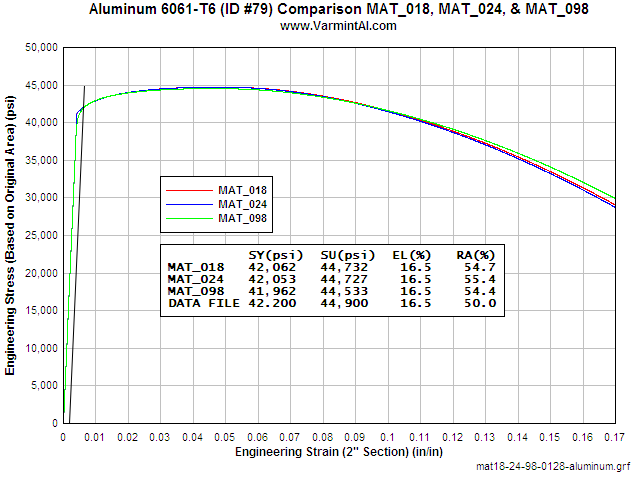
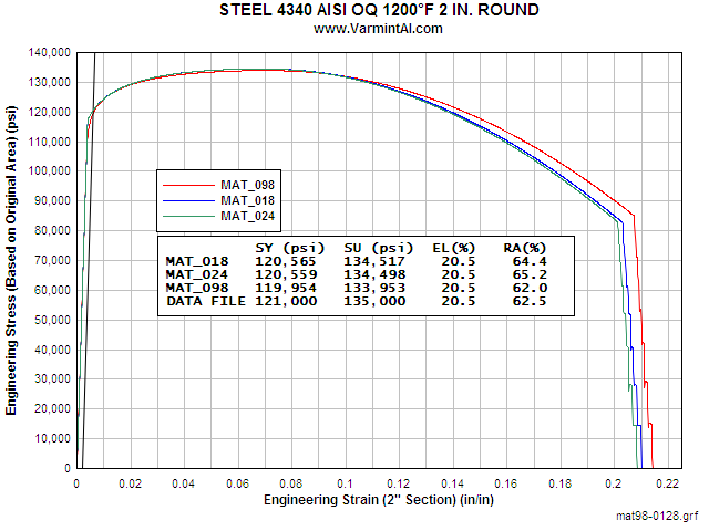
VERIFYING MAT_098.... The object of this calculation was to verify that MAT_098 would reproduce the input material data from a simulation of a Tensile Test. The FEA geometry is that of a Standard 1/2" Tensile Test that is used to measures the mechanical properties of metals. The calculation runs in the 3D implicit mode with the extension applied in 0.0001 inch increments. The resulting load was then calculated with LS-PrePost using the bndout ASCII file. The mesh consists of 13,294 nodes and 11,700 solid 8-node brick elements. The run time is about 5 hours on my 2.8 GHz Athlon II X4 64 computer. The calculation could be completed in a much shorter time, but the fine increments of displacement were used in order to make a smooth stress-strain curve. If you would like to run the calculation yourself here is the LS-DYNA Keyword input file: Download aluminum-6061-t6-mat98-run.zip (277Kb) It is setup to run with aluminum 6061-T6 in English Units and it is very easy to copy and paste a different material of interest.
THE "A" PARAMETER.... The "A" parameter of the Johnson-Cook Plasticity Model equation (S = A + B * epN) has been typically taken as the engineering yield stress. By fixing "A" to that value it was not possible to reproduce the Standard Tensile Test results similar to the input material properties. Much better results were obtained by allowing "A" be a much lower value. It appears that "A" best fits the data when it is approximately the elastic limit of the Engineering Stress/Strain curve. The material properties in the Database are for low strain rates. Since high strain rate information is not available it is left to the user to supply the high strain rate parameters. The A, B, and N values also apply to the MAT_15 (*MAT_JOHNSON_COOK).
Aluminum 6061-T6 Tensile Test
Simulation with MAT_098
Simplified Johnson-Cook Plasticity Model
The chart shows the calculated Engineering Stress vs Strain in a two inch gauge length of the LS-DYNA Tensile Test simulation. The Simplified Johnson-Cook Plasticity model reproduces the input properties with good accuracy. The largest error is in the Reduction in Area. In an actual tensile test specimen measuring the diameter at the fracture location is difficult to do accurately. The agreement here is well within the range that is normally expected between samples of the same material. The tensile test simulation was also done for steels 4140 & 4340 with similar results.
Table 3: Comparison of the
Aluminum 6061-T6 Results to the Input Material Properties
for the Johnson-Cook Plasticity Parameters.
| Material Property | Input From the MAT_098 Database | LS-DYNA Calculated Property from the FEA Simulated Tensile Test | Error |
| Modulus of Elasticity | 10,000,000 psi | 9,956,022 psi | 0.26% |
| Engineering Yield Stress | 42,200 psi | 42,098 psi | 0.27% |
| Engineering Ultimate Stress | 44,900 psi | 44,716 psi | 0.41% |
| Elongation at Failure | 16.5% | 16.2% | 1.82% |
| Reduction in Area | 50% | 52.4% | 4.8% |
Table 4: Material Property input in the MAT_098 Tensile Test Simulation
*MAT_SIMPLIFIED_JOHNSON_COOK |
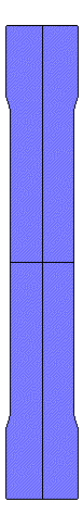
 Mesh as used with 3 planes of symmetry |
 Mesh reflected to show shape |
 Mesh showing necking |
Fine mesh detail.
Download the fine Tensile Test Mesh input Keyword file ready to run
here.
Plasticity With Failure Strain
 |
|
Effective Plastic Failure Strain MAT_098 &
MAT_018
LS-DYNA 3D mesh MAT_018 & MAT_098 with Effective Plastic
Failure Strain

LS-DYNA 3D mesh MAT_018 & MAT_098 with Effective Plastic
Failure Strain
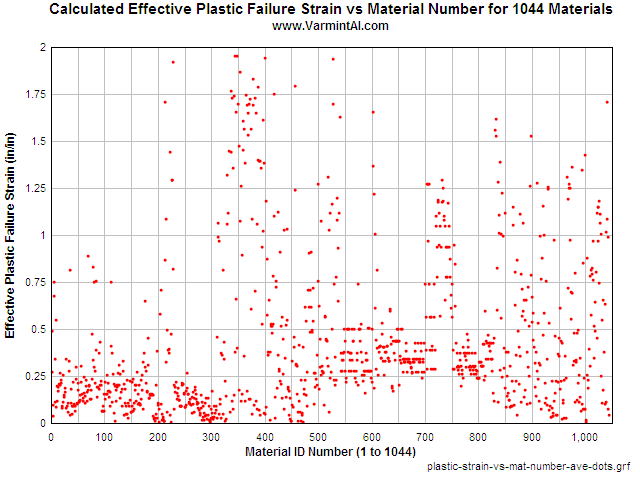
Note: Two materials are off the chart. Polycarbonate and
Teflon.
Three Methods of Calculating Effective Plastic Failure Strain.
The effective plastic strain at failure for a material is typically not included in any material property databases. It was not included in the Database of 1044 materials that I collected over the years. However it was possible to calculate the Effective Plastic Failure Strain (epfs) from the given data. I am aware of three methods to calculate effective plastic failure strain.
Method 1. Plastic failure strain (not the total strain) can be calculated from the given percent Reduction in Area (RA) value in the database by using the RA equation below and this method was not used.
epfs = ln ( 100 / (100 - RA))
The equation assumes a uniform plastic strain across the section, from the center line to the surface, where the necking occurs. The LS-DYNA calculations show that the highest effective plastic strain occurs at the center line of the tensile test specimen at failure and decreases as one moves toward the surface. Only 287 of the materials in the database include the value for the percent Reduction in Area. The RA in the database is usually a rough measurement on a broken specimen made with calipers. The measurement is not the same dimension as it would be under load. As failure occurs while testing the first area where incipient failure occurs is in the center of the section. As the tensile specimen continues to fail, the ruptured area is further distorted.
Method 2. The effective plastic failure strain was calculated with LS-DYNA. A tensile test specimen can be loaded, in an implicit 2D calculation, and the epfs can be determined by observing the maximum epfs when the diameter at the neck matches the diameter given for RA. This method works well if RA data is available and is probably a better estimate of epfs than merely using the RA equation. This requires a separate LS-DYNA run for each material that includes the RA in the database.
Method 3. This method to calculate the epfs with LS-DYNA requires running the tensile test simulation but within certain conditions. It requires a separate LS-DYNA run for each material that includes the elongation in the database. When the calculated elongation matched the database value, the center element at the neck is at the epfs. This method works well with materials that exhibit a diffuse necking over a long section of the specimen. But it over estimates the epfs when a very short localized neck is observed. The specimen's diameter at the neck can end up being very small value with extremely distorted elements. The accuracy with these distorted elements is poor and some of these materials have indicate an epfs greater than 2.0 in/in. In a second series of calculations on each material I did the following. If the RA was not available I assumed it to be no larger than 75% or equivalent to a 0.25 inch diameter at the smallest section of the neck.
The procedure I used is was to first calculate the epfs for all 1044 materials based on elongation or RA only if available. Then for those materials that did not include RA, another calculation was completed limiting the RA to no more than half the original 0.5" diameter (RA = 75%). Finally I took the average of the two results as the effective plastic failure strain epfs for each material. For values of epfs greater than ~1.5 in/in the accuracy is poor. Reasonably sized elements would be greatly distorted and the results should be used with caution.
To implement the computer runs, I used a DOS BATCH file to submit each calculation automatically and rename the elout file with the correct material list number. Running 1044 materials took about 52 hours CPU time for each of the two runs. Computers work tirelessly and don't complain as long as power is supplied.
The effective plastic failure strain is included in the new material property files for MAT_018, MAT_024, and MAT_098. The most recent version of LS-DYNA will include the plastic failure strain capability for MAT_018 and MAT_024. Plastic failure strain is already implemented for MAT_098 but not for 2D implicit calculations.
The files contain the 5 systems of units in one zip file including a matlist.txt file which lists the material by number. The numbering system makes it easier to browse the list and later select a material by number from the database. The epfs is included for each material in the proper field for copying and pasting into a K-File for LS-DYNA.
Comparison of the calculated Engineering Stress Strain curve for
three material models of 4340 Steel.![]()
The user can calculate a similar Stress Strain curve for any one of
the 1044 materials using this input KEYWORD file.
It is setup for MAT_018 as is, but it is easy to replace the
material with one of your choice for either MAT_018,
MAT_024, or MAT_098. Download the mesh zip
file here: pull3dspin-run.zip The
run time on my computer
is about 26 minutes with the very fine implicit load steps.
How do MAT_018 & MAT_098 Compare
to the old BASIC code?

Download the bolts.exe calculator. It runs in a DOS box.
  Grade 8 10/32 cap screw loaded to failure Fringes of Effective Plastic Strain |
 Failure starts at the thread roots and finally proceeds from the center out. One can see the elements deleted as they exceed the Effective Plastic Failure Strain (epfs). |
 Fine 2D Mesh Detail (View reflected about center line) |
 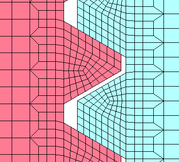 Thread Mesh Detail Zoom |
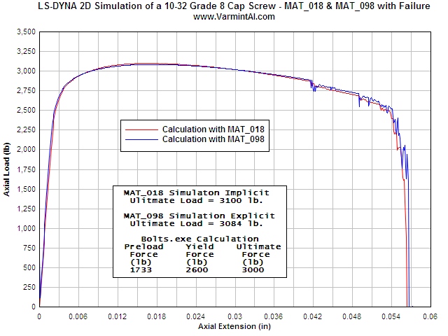
The axial load vs bolt extension. At large extensions, the threads
start to fail at the thread root. Finally
the center 2 elements exceed the failure strain and are deleted
from the mesh. As the extension
increases the neighboring elements fail until complete separation
occurs.
![]()
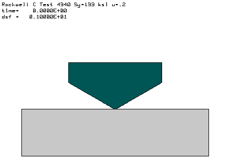
POWERFUL TOOL.... The NIKE2D Finite Element Code by Livermore Software Technology Corp is a very powerful 2-D tool for calculating the loads and deformations of axisymmetric structures. Often, I need to know the yield and ultimate stress of materials when given only the Rockwell C hardness. NIKE2D can be used to calculate the Rockwell C hardness of various materials in the material.txt Database. Being able to calculate the Rockwell C hardness of a steel is very useful in selecting the correct material properties for a material of interest.
THE MEASUREMENTS.... I have generated a 2-D FEA model of the the Rockwell hardness testing procedure. The diamond cone, used for the Rockwell C hardness testing, has a 120 degree included angle with a 0.02 mm tip radius. In the calculation, the loading is identical to the actual test procedure. A 10 Kg load is applied to the diamond, the displacement if the diamond indenter is recorded and then the load is increased to 150 Kg. The load is then decreased back down to 10 Kg and the displacement of the diamond is again recorded. These two measurements are used to calculate the Rockwell C hardness. A friction coefficient of 0.2 is used between the diamond surface and the steel.
THE MATH.... The difference of the first 10 Kg load depth and the second 10 Kg depth, measured in millimeters divided by 0.002 mm and then subtracted from 100 is the Rockwell C hardness.
Rc = 100 - (Y2 - Y1) / 0.002
|
1. The diamond cone is loaded to 10 Kg and the
vertical displacement is recorded (Y1). |
Table 1: Hardness numbers for 4340 Steel in various heat treat conditions.
| Steel 4340 Yield Stress (psi) |
Nominal Rockwell C |
Calculated Rockwell C u=0.2 |
Nominal Brinell Hardness |
Calculated Brinell Hardness |
| 69,000 | 13.07 | 217 | ||
| 90,000 | 18 | 20.54 | 220 | |
| 121,000 | 27 | 28.65 | ||
| 128,000 | 28* | 29.12 | 270 | |
| 133,000 | 30.72 | |||
| 135,000 | 28* | 32.33 | 310 | |
| 150,000 | 37 | 35.07 | 340 | |
| 159,000 | 36 | 35.54 | ||
| 170,000 | 39.70 | 380 | ||
| 185,000 | 43 | 42.47 | 400 | |
| 200,000 | 43.69 | 430 | ||
| 238,000 | 49.86 | 550 | ||
u = 0.2 is the friction coefficient between the
diamond and the test metal.
* The available data is obviously not very accurate in the midrange
of yield stresses.
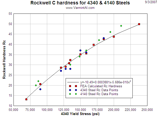
The Rc calculated hardness fits the available data reasonably
well.
When time allows, I will generate another FEA model to calculate the Brinell hardness metals. I recently found data on 4140 steel and added it to the plot. The calculations were only for 4340 steel, but they look very similar.
Material Name and Condition.            Density Yng's Poiss  Yld   Ult  Elong Redu CTE   Yld
                                        lb/in^3 Modul Ratio  Strs  Strs   %   Area 10^-6 off-
                                                 msi         ksi   ksi         %   /degF set
steel wrought 4340 1 in. bar annealed    0.2830 30.00 0.290  69.0 108.0  22.0 50.0  6.30 0.20
steel wrought 4340 Case 1                0.2830 30.00 0.290  90.0 117.8  21.4 54.0  6.30 0.20
steel wrought 4340 Case 2                0.2830 30.00 0.290 128.0 143.2  18.4 56.0  6.30 0.20
steel wrought 4340 1 in. bar oq+1200f    0.2830 30.00 0.290 133.0 147.0  18.0 57.0  6.30 0.20
steel wrought 4340 Case 3                0.2830 30.00 0.290 135.0 149.1  17.7 54.0  6.30 0.20
steel wrought 4340 Case 4                0.2830 30.00 0.290 150.0 163.2  16.8 53.0  6.30 0.20
steel wrought 4340                       0.2840 29.70 0.290 159.0 165.0  16.5 54.1  6.83 0.20
steel wrought 4340 1 in. bar oq+1200f    0.2830 30.00 0.290 170.0 183.0  14.0 52.0  6.30 0.20
steel wrought 4340 Case 5                0.2830 30.00 0.290 185.0 203.0  12.9 48.0  6.30 0.20
steel wrought 4340 1 in. bar oq+800f     0.2830 30.00 0.290 200.0 222.0  12.0 47.0  6.30 0.20
steel wrought 4340 1 in. bar oq+400f     0.2830 30.00 0.290 238.0 283.0  11.0 48.0  6.30 0.20
steel wrought 4140 1 in. bar annealed    0.2830 29.00 0.290  61.0  95.0  26.0 57.0  6.20 0.20
steel wrought 4140 1 in. bar norm        0.2830 29.00 0.290  95.0 148.0  18.0 47.0  6.20 0.20
steel wrought 4140 1 in. bar oq+1200f    0.2830 30.00 0.290  95.0 110.0  18.0 53.0  6.20 0.20
steel wrought 4140 1 in. bar oq+1000f    0.2830 30.00 0.290 143.0 165.0  15.0 50.0  6.20 0.20
steel wrought 4140 1 in. bar oq+400f     0.2830 30.00 0.290 238.0 257.0   8.0 38.0  6.20 0.20
![]()
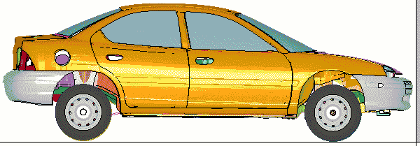
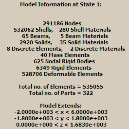
Neon Crash Test Benchmark Calculation
LS-DYNA Benchmark Tests for Four
Computers
Neon_Refined_Revised Benchmark Calculation.
|
Computer |
Precision |
No. CPU's |
Memory Used |
Time/Zone Cycle |
Total CPU Time |
Relative Time |
| Y-Mach Windows XP |
Single | 1 | 77,294,865 | 630 | 10,140 | 2.950 |
| Single | 2 | 79,102,659 | 334 | 5,369 | 1.562 | |
| Single | 3 | 80,849,823 | 251 | 4,027 | 1.172 | |
| Single | 4 | 82,596,987 | 214 | 3,437 | 1.000 | |
| Double | 4 | 78,223,374 | 437 | 7,012 | 2.040 | |
| 7-Mach Windows 7 64-bit |
Single | 1 | 77,265,367 (4-bytes) |
596 | 9,592 | 2.791 |
| Single | 2 | 79,073,161 (4-bytes) |
345 | 5,564 | 1.619 | |
| Double | 2 | 74,699,548 (8-bytes) |
590 | 9,497 | 2.763 | |
|
Base-Computer |
|
|
|
|
|
|
|
|
|
|
|
|
|
|
|
Double |
4 |
88,548,197 |
122 |
1,975 |
0.281 |
|
|
T-Mach |
Single |
1 |
77,294,975 |
1,169 |
18,736 |
5.451 |
| Single | 2 | 79,102,769 (4-bytes) |
1,154 | 18,522 | 5.389 | |
| Double | 2 | 74,729,156 (8-bytes) |
2,146 | 34,478 | 10.031 |
*The New Base-Computer with the Ryzen CPU is 3.56
times faster than
the fastest Windows XP computer
 .
.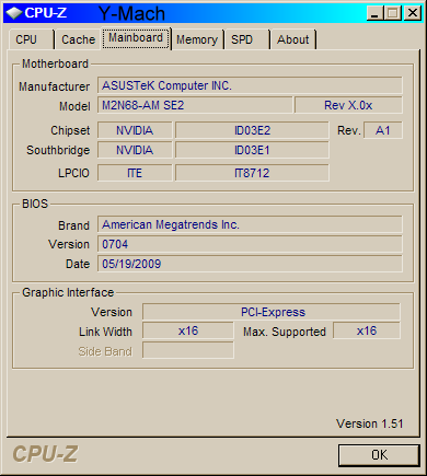
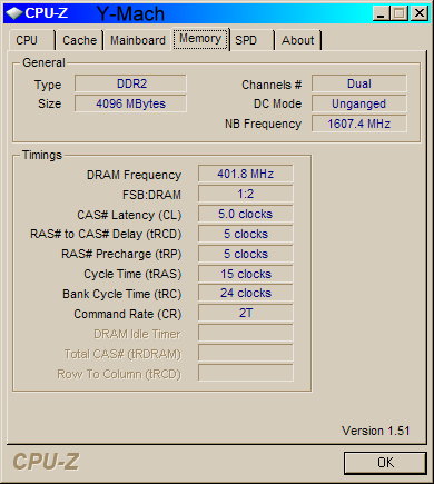
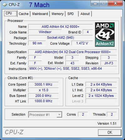
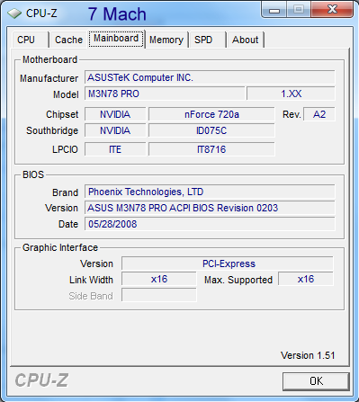
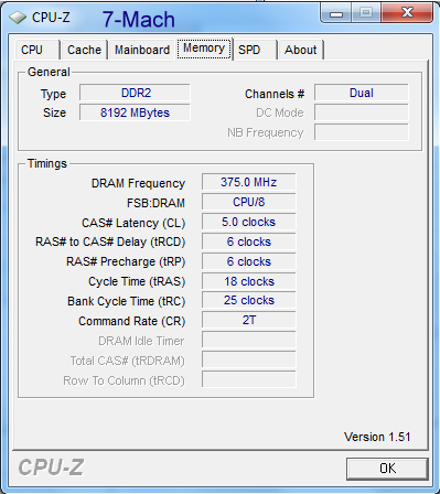
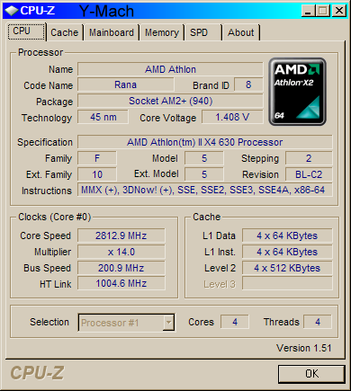
The above three screen shots show the information on my 7-Mach
computer recently assembled and running the Windows 7 64 bit
Release Candidate. LS-DYNA ran the benchmark test very well. I did
have to set the Energy Management to "never" turn of the computer
or monitor. Windows 7 is looking good, but DIFFERENT!

Top Crunch FEA Benchmark Problem Downloads plus Results for numerous computers.
Movie of the Neon_Refined_Revised Benchmark Calculation.
Car traveling at 35 mph hitting a rigid wall. The calculation ends
at 30 ms.
Note: To make a better movie I made a special run with more plot
states.
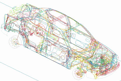
Part edges to show the extensive detail of the model.
![]()
 You can purchase quality
materials from Online Metals in any
quantities/sizes.
You can purchase quality
materials from Online Metals in any
quantities/sizes.
![]()
Table 1: Summary of the example problems
|
Problem Name |
Material No. |
Sliding interface |
Pressure loading |
Displacement loading |
Thermal loading |
Unloading |
Failure |
Threads |
Other |
|
I357 |
13 |
4 |
V-zero |
||||||
|
CUTV |
13 |
4 |
y |
y |
V-zero |
||||
|
ADISK4 |
10 |
y |
|||||||
|
B440 |
10 |
4 |
y |
y |
y |
||||
|
BDISK |
10 |
4 |
y |
y |
|||||
|
BELLOW |
10 |
y |
y |
y |
|||||
|
BELLV1 |
1,10 |
4 |
y |
y |
|||||
|
CAP25 |
10 |
4 |
y |
y |
y |
||||
|
CORE |
10 |
y |
|||||||
|
COREWP |
10,12 |
4 |
y |
y |
y |
||||
|
COREHP |
10,12 |
4 |
y |
y |
y |
||||
|
FILLP |
7,10 |
4 |
y |
y |
y |
y |
Preload |
||
|
LEVEE |
1,5 |
1 |
G loading |
||||||
|
NOZZ2DF |
1 |
Modal |
|||||||
|
OLDWELDA |
1,12 |
4 |
y |
Residual St. |
|||||
|
PCUTW |
7,10 |
4 |
y |
y |
y |
y |
|||
|
PISTON |
10 |
y |
y |
y |
|||||
|
PISTON1 |
10 |
y |
y |
y |
|||||
|
PRIMER |
10 |
4 |
y |
y |
y |
||||
|
PULLA |
10 |
y |
y |
||||||
|
RDISK |
10 |
4 |
y |
y |
|||||
|
RIVET |
3 |
4 |
y |
y |
y |
Plastic flow |
|||
|
SHEET22 |
10 |
4 |
y |
y |
y |
||||
|
SNAP |
10 |
3 |
y |
y |
|||||
|
SPRING |
1,10 |
4 |
y |
y |
|||||
|
TANKW45 |
10 |
4 |
y |
y |
y |
||||
|
TUNE |
1 |
Modal |
|||||||
|
WASH |
10 |
4 |
y |
y |
|||||
|
WIRE |
10 |
3 |
y |
y |
|||||
|
BASE9F |
1 |
Modal 3D |
|||||||
|
BASE9Z |
1 |
G Loading |
|||||||
|
BASE9X |
1 |
G Loading |
|||||||
|
CHAIN10 |
9 |
y |
|||||||
|
GLI |
1 |
Modal 3D |
|||||||
|
NOZZ7 |
4 |
y |
Thermal 3D |
||||||
|
GTANK100 |
3 |
y |
Convection |
||||||
|
I100TANK |
3 |
y |
Convection |
||||||
|
TTWAYA |
3 |
4 |
y |
Heat-Gen. |
|||||
|
TWAYH |
3 |
4 |
y |
Heat Gen. |
Brief description of most of the example problems listed in the table:
DYNA2D
I357 This is a 357 magnum bullet traveling at 1000 fps and impacting a copper plate. There is a type 4 sliding interface between the bullet and the plate.
CUTV This is a high explosive actuated valve cutting a 20 mil thick stainless steel burst disk. The disk has 9000 psi of gas pressure behind it. The force acting on the cutting end of the plunger is much less than the approximately 4000 lb of driving force of the cutter.
NIKE2D
ADISK4 This is an analysis of a machined burst disk to determine the burst pressure.
B440 This is the analysis of a high strength 4-40 heat treated cap screw under axial load. The thread form is standard UNC sized for minimum material condition. The load is applied by a displacement boundary. The thread contact is implemented with the type 4 sliding interface with a 0.3 friction factor to simulate clean, dry threads. The failure load agrees with the minimum tested tensile strength listed in the specifications. The bolt material is implemented with the material model number 10, which is the power law hardening isotropic plasticity material model. The STRAIN code was used to format the material properties and then a block copy was used to insert the material properties in the NIKE2D input deck.
BDISK This is a simple fine mesh burst disk bending over the sharp corner of the bore diameter of the backup piece. A sliding interface between the disk and the support allows sliding between the disk and the backup piece. There is a conical dimple at the center of the burst disk. Even with the sharp corner, the highest stresses and failure occur at the center of the disk.
BELLOW This is a thin wall bellows that is under simultaneous axial extension and internal gas pressure. The pressure capability decreases as the axial extension increases.
BELLV1 This is a belleville spring washer being compressed between two plates. The contact between the washer and the plates is implemented with type 4 sliding interfaces and the load is applied with a displacement boundary on the top plate. The displacement boundary loading is more stable than a pressure boundary loading. The forces at a given displacement can readily be found while post-processing with ORION. This particular spring cannot be loaded to the flat position and remain elastic. For the spring to remain elastic, this spring should be redesigned.
CAP25 This is a 1/4-20 UNC high strength heat treated cap screw with nominal dimensions. It is similar to B440. I have written a small BASIC program that uses Machinery's Handbook data and generates the thread form MAZE line definitions for any standard UNC, UNF, or UNEF thread.
CORE This is an annealed aluminum weld bead under gas pressure loading.
COREWP This a titanium weld with the weld residual stress state simulated by a thermal cool-down of the weld bead. After cool-down, the pressure is applied to determine the failure pressure. The time step needs to be increased by typing SW6. after a time of 1.0 when the weld bead cool-down is complete. The weld bead is merged to the base metals "by hand" in a node by node process in the maze input deck.
COREHP This is a problem similar to COREWP, but with a leaking burst disk. By allowing gas pressure on both sides of the burst disk, the pressure capability of the fitting, after the disk bursts, can be calculated.
FILLP A threaded fitting is given a preload force that would result from the assembly torque and then loaded with an internal gas pressure. The thermal expansion of a number of elements in the load path are forced to expand thermally with material model #7. The CTE of the thermal material is adjusted to give the correct preload force that the assembly torque would produce. When the gas pressure is applied, the preload force is reduced as the pressure is increased. The pressure that caused a zero contact force can be calculated and at higher pressures, the gap at the contact surfaces can be calculated. This is a very powerful method of analyzing pressure fittings.
LEVEE This problem is a plane strain section of an earth levee or dam with water on one side and a three-to-one slope on the other side. The loading is a one G vertical acceleration. The location of peak shear stress in the levee indicates where possible failures could occur at high tide. The soil is implemented with material model #5. Three sided parts are used in the MAZE input deck.
NOZZ2DF The axisymmetric mode shapes and natural frequencies are found for a thruster nozzle fixed at its base.
OLDWELDA The first weld design failed due to the weld residual stresses and the location of the weld undercut. This calculation uses the thermal material model #12 and temperature dependent material properties to calculate the residual weld stresses during the weld bead cool-down.
PCUTW The preload resulting from the assembly torque is applied with a row of thermal elements modeled with material #7. After one time step, the preload is applied. SW6. is used to change the time step to 1000 or a reasonable gas pressure increment. Gas pressure is increased until failure occurs. Failure occurs when NIKE2D is unable to find an equilibrium condition for the next increment of pressure. At failure, the thread relief section of the fitting separates when plastic instability occurs. Plastic instability occurs when a small increase in pressure causes the load at the thread relief section to increase at a greater rate, both due to the increased pressure and to the reduced thread relief section, as it necks, than the material can increase its strength, as it strain hardens. At the 26,000 psi failure pressure, the gap at the seating surfaces is 7 mils and the "O" ring would be extruded because it could not possibly maintain a seal at such a high pressure with such a large gap.
PISTON This is a thin wall piston inside a thin wall tube. The piston has an "O" ring at each end and the analysis was used to calculate the pressure at which the center of the piston deforms and contacts the tank wall.
PISTON1 is a design with a stiffening ring in its center that functions at the higher pressure without contacting the tank wall. Two nodes on the inner surface of the piston were moved by hand to create the stiffening ring.
PRIMER This is a rifle primer being dented and pressurized during the firing of a rifle. The firing pin dents the primer cup and then a 55,000 psi internal pressure is applied and removed. The firing pin is then extracted to get the final shape. Loading is controlled with two separate load curves. The final shape agrees with a standard load in a 243 Winchester cartridge.
PULLA This is a test of material model #10. The properties for aluminum 6061-T6 are input into the STRAIN code to calculate the constants for the material model. A standard pull specimen is loaded to failure with NIKE2D. The 0.2% offset yield stress and the ultimate engineering stress are calculated with NIKE2D and plotted with ORION.
Sy = 42,200 psi input data
Su = 44,900 psi input data
Sy = 42,277 psi calculated with NIKE2D
Su = 44,945 psi calculated with NIKE2D
RDISK This is a 2 mil thick burst disk machined into a stainless steel slug that is similar to BDISK. The failure pressure is 4600 psi where plastic instability occurs.
RIVET This is the forming of a mild steel rivet to fasten two plates together. The rivet fills the hole and has a high axial preload after forming. The sliding interface #4 is used between contacting surfaces. After the rivet is formed, the rivet set is lifted. For a better design, the rivet set should be more of an elliptical shape to cause a larger diameter rivet head. This calculation uses the "auto" command on card #1 to allow NIKE2D to select the optimum time step size and to automatically restart if a time step is too large.
SHEET22 This is a copper burst disk clamped in place with a steel bull-nose clamp. This burst disk requires no machining like the earlier problems and can be punched out by the gross. The first two time steps only apply the clamping force. Typing SW6. allows the changing of the time step to 100 psi, which is a reasonable pressure increment. The clamping force is maintained with a constant displacement during the application of the gas pressure. The burst pressure can be adjusted and calculated simply by changing the bore diameter of the backup ring.
SNAP This is a calculation to determine the snap ring's ability to support an axial load produced by a gap pressure. The snap ring is implemented with material model #14 (circumferentially cracked isotropic/kinematic plasticity). Sliding interface #4 with friction was used at the contact surfaces.
SPRING This is a truck leaf spring that is loaded by displacing the pinned end and holding the center section fixed. After displacing 5 in., the displacement is forced back to its initial position. There is plastic deformation in the bottom leaf. The load deflection curve for the spring is plotted. The calculation uses sliding interface #4 with friction between the leaf sections and type #3 at the lubricated pinned end. The pin is free to rotate relative to the end of the spring.
TANKW45 This is a titanium tank with a threaded end cap. Internal gas pressure is sealed at the first "O" ring and the end cap loads the threads. This analysis also uses a type #4 sliding interface between all contacting surfaces. The tank fails by expelling the end cap as the threads rotate and slip free.
TUNE This is a musical tuning fork for tuning to the "A" tone (440 Hz). The fork is magnetic and assumed to be steel. The dimensions were measured with a micrometer. NIKE2D calculates the first mode shape to have a natural frequency of 465 Hz, or an error of 3.7%.
WASH This is a large washer with an edge load.
WIRE This is a calculation of one of the forming processes in making a wire. The initial condition of the wire is annealed copper. The wire is pulled through the die at a tensile force of 45 lb. The sliding interface #3 between the die and wire simulates a lubricated die.
If you are interested in more information on some of these examples or would like the MAZE input and/or output file, send me email.
![]()
Comprehending Engineers - Take One
Two engineering students were walking across campus when one said,
"Where did you get such a great bike?" The second engineer replied,
"Well, I was walking along yesterday minding my own business when a
beautiful woman rode up on this bike. She threw the bike to the
ground, took off all her clothes and said, "Take what you want."
"The second engineer nodded approvingly, Good choice; the clothes
probably wouldn't have fit."
Comprehending Engineers - Take Two
To the optimist, the glass is half full. To the pessimist, the
glass is half empty. To the engineer, the glass is twice as large
as necessary.
Take 2.50: To the engineer, the capacity of the container has
been over designed by a factor of approximately 1.905 assuming a 5%
volume for the sloshing safety factor.
Comprehending Engineers-Take Three
A pastor, a doctor and an engineer were waiting one morning for a
particularly slow group of golfers. The engineer fumed, "What's
with these guys? We must have been waiting for 15 minutes!" The
doctor chimed in, "I don't know, but I've never seen such
ineptitude! "The pastor said, "Here comes the greens keeper, let's
have a word with him. " (dramatic pause) "Hi George. Say, what's
with that group ahead of us? They're rather slow, aren't they?" The
greens keeper replied, "Oh, yes, that's a group of blind
firefighters. They lost their sight saving our clubhouse from a
fire last year, so we always let them play for free anytime." The
group was silent for a moment. The pastor said, "That's so sad. I
think I will say a special prayer for them tonight." The doctor
said, "Good idea. And I'm going to contact my ophthalmologist buddy
and see if there's anything he can do for them." The engineer said,
"Why can't these guys play at night?"
Comprehending Engineers - Take 4
There was an engineer who had an exceptional gift for fixing all
things mechanical. After serving his company loyally for over 30
years, he happily retired. Several years later the company
contacted him regarding a seemingly impossible problem they were
having with one of their multimillion dollar machines. They had
tried everything and everyone else to get the machine to work but
to no avail. In desperation, they called on the retired engineer
who had solved so many of their problems in the past. The engineer
reluctantly took the challenge. He spent a day studying the huge
machine. At the end of the day, he marked a small "x" in chalk on a
particular component of the machine and stated, "This is where your
problem is". The part was replaced and the machine worked perfectly
again. The company received a bill for $50,000 from the engineer
for his service. They demanded an itemized accounting of his
charges. The engineer responded briefly...
One chalk mark:
$1
Knowing where to put it:
$49,999.
It was paid in full and the engineer retired again in peace.
Comprehending Engineers-Take Five
What is the
difference between Mechanical Engineers and Civil Engineers?
Mechanical Engineers build weapons, Civil Engineers build
targets.
Comprehending Engineers-Take Six
The graduate with a
Science degree asks, "Why does it work?"
The graduate with an Engineering degree asks, "How does it
work?"
The graduate with an Accounting degree asks, "How much will it
cost?"
The graduate with a Liberal Arts degree asks, "Do you want fries
with that?"
Comprehending Engineers-Take Seven
"Normal people ... believe that if it ain't broke, don't fix it.
Engineers believe that if it ain't broke, it doesn't have enough
features." ----- Scott Adams, The Dilbert Principle
Comprehending Engineers-Take Eight
An artist, an
architect and an engineer were discussing whether it was better to
spend time with the wife or a mistress. The architect said he
enjoyed time with his wife, building a solid foundation for an
enduring relationship. The artist said he enjoyed time with his
mistress, because of the passion and mystery he found there. The
engineer said, "I like both." "Both?" Engineer: "Yeah. If you have
a wife and a mistress, they will each assume you are spending time
with the other woman, and you can go to the lab and get some work
done!"
|
ENGINEERS AND SOCIAL SKILLS "Normal" people expect to accomplish several unrealistic things from social interaction:
In contrast to "normal" people, engineers have rational objectives for social interactions:
FASCINATION WITH GADGETS Clothes are the lowest priority for an engineer, assuming the
basic thresholds for temperature and decency have been satisfied.
If no appendages are freezing or sticking together, and if no
private parts or mammary glands are swinging around in plain view,
then the objective of clothing has been met. Anything else is a
waste.
Female engineers become irresistible to male engineers at the
age of consent and remain that way until, oh, about their clinical
death.
FRUGALITY
The risk/reward calculation for engineers looks something like this:
Being practical people, engineers evaluate this balance of risks
and rewards and decide that risk is not a good thing. The best way
to avoid risk is by advising that any activity is technically
impossible for reasons that are far too complicated to explain. If
that approach is not sufficient to halt a project, then the
engineer will fall back to a second line of defense: "It's
technically possible but it will cost too much."
The fastest way to get an engineer to solve a problem is to
declare that the problem is unsolvable. No engineer can walk away
from an unsolvable problem until it's solved. No illness or
distraction is sufficient to get the engineer off the case. These
types of challenges quickly become personal -- a battle between the
engineer and the laws of nature. (Source Unknown. But whoever it was, had inside info on engineers.) Mary Ann's Reply to the above:
|
Engineering requires an understanding of mathematics
|
Teaching Math through the decades* Last week a I purchased a burger for $1.58. I handed the cashier
$2.00 *(Found this on the web in a number of locations. I didn't write
it.) |
Last Updated:
10/2/2021
End of Page![]()